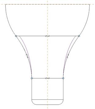
When we click on the blue check mark, we see the following preview.
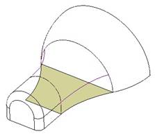
Click on the green check mark to complete the feature. Now, we have two surfaces that are not connected, so we will need to merge them together. Change over to the Quilts selection filter, pick both surfaces (using Ctrl), and merge them together. You should now be left with a single quilt in the middle with purple internal edges. The only pink edges are the ones that touch the solid volumes on either end, as shown in the next figure.
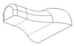
Now we can solidify the model. Click on the single quilt surface in the middle so it highlights, as shown in the next figure.
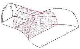
Next, click on the Solidify tool. Initially we see the following preview.
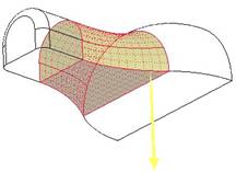
If we look in the dashboard, we can see that the Patch option is selected, as shown in the following figure.
![]()
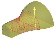
We want to switch over to the Solid option (the first icon all the way to the left), and then flip the yellow arrow so it points into the model. The preview should now show the entire model highlighted, as shown in the next figure.
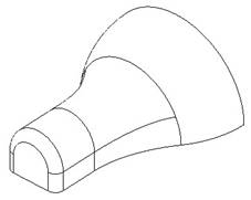
Click on the green check mark to complete the solidify tool, and we should be left with a completely solid model, as shown in the next figure.
Save and close this model.
LESSON 30 – Thicken Tool
Open up the Project_Exercise model again, which looks like the following if all previous lessons have been completed.
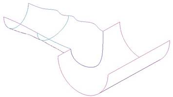
The first thing we are going to do is add a round to the intersection of these two surfaces. Therefore, click on the Round tool, enter 0.25” for the radius, and pick the following edge.
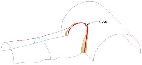
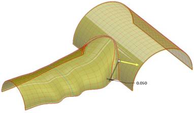
Complete this round. Now, switch over to the Quilts selection filter, and pick on the entire surface model. Once the entire model is highlighted, click on the Thicken tool. In the dashboard, enter 0.05” for the thickness, and flip the arrow if necessary to get it to the inside. The preview for the thicken tool should look like the following.
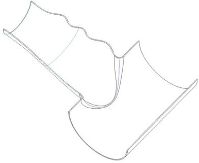
Complete this tool, and the model will look like the following.
Save and close this model.
LESSON 31 – Extend Tool
Open up the Extend2 model, which looks like the following figure.
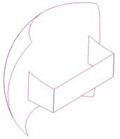
We are going to start by setting our selection filter to Geometry, and then we are going to pick on the following surface edge.
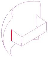
Once the edge is selected, click on the Extend tool. We will see a preview for the extend, as shown below.
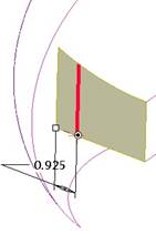
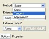
Before we extend this out we will go to the Options slide-up panel and change the type from Same to Tangent, as shown in the next figure.
Now, change the extend distance to 3.5, which should clear our domed surface, as shown in the next figure.
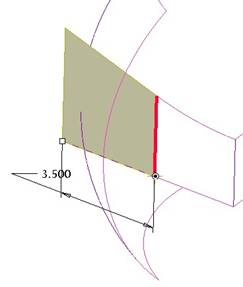
Click on the green check mark to complete this first extend. Repeat this process for the other side, to arrive at the following.
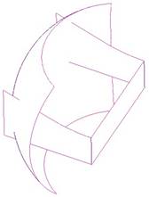
Now that we have both sides extended, we will switch over to the Quilts selection filter, and pick both quilt surfaces. Click on the Merge tool, and you will get the following.
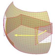
If your preview looks like the one above, click on the green check mark to get the following quilt surface.
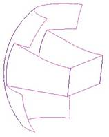
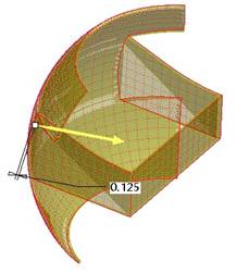
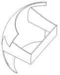
Click on the entire quilt surface, and then select the Thicken tool. Flip the arrow so it is pointing into the inside of the surface, and change the thickness to 0.125”. The following figure shows the preview for this.
Click on the green check mark, and our part is completed, as shown in the next figure.
Save and close this model.
LESSON 32 – Mirror Tool
Funnel
Open up the funnel model that we worked with in an earlier lesson. It looks like the following.
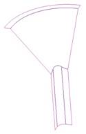
Since this is a surface model, we will mirror the surface instead of the entire part. The advantage of mirroring individual features is that it does not mirror the default datum geometry or anything else, just the surface. Therefore, we will use the Quilts selection filter, and pick on the single quilt.
Once the quilt is selected, click on the mirror tool, or go to Edit, Mirror from the menu bar. When the dashboard appears, click on the FRONT datum plane to mirror about. We will see the following preview.
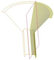
Click on the green check mark to complete this mirror, and then merge the two surfaces together using the Merge tool. The result will be the following.
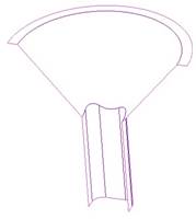
Now, pick this entire surface, followed by the Mirror tool again, and then pick on the RIGHT datum plane. The preview looks like the following.
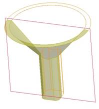
Complete this mirror, merge the two sides together, and you will have your final funnel part.
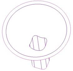
Save and close this part.
BBS2
Open up the BBS2 part. Since this is a solid model, we will mirror the entire part. Therefore, in the model tree, select on the BBS2.PRT words at the top of the tree. Once you have selected this, click on the Mirror tool.
When the dashboard appears, use the TOP datum plane to mirror about, and you will see the following preview.
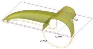
Click on the green check mark to complete this mirror. Hide the mirror in the model tree to eliminate any extra curves, planes, etc. that may have been in the first side. The following figure shows this completed model.
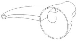
Save and close this model.
Project_Exercise
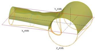
Open up the Project_Excercise model. It too is a solid model, so we will select the entire model by picking on its name in the model tree, followed by the Mirror tool. For a mirroring plane, pick on the TOP datum plane again. The following shows the preview for this mirror.
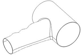
The completed part will look like the next figure.
Save and close this model.
Extend1
Open up the Extend1 model that we worked with earlier. It should currently look like the following.
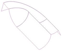
The first thing we are going to do is mirror this surface. Therefore, use the Quilts selection filter, and pick the entire surface, followed by the Mirror tool. For a mirroring plane, select the RIGHT datum plane. We will see the following preview.
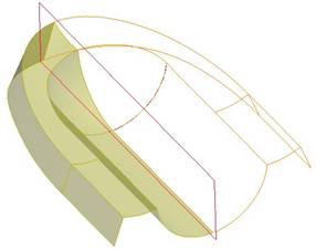
Once you mirror the surface, perform a merge operation to create one larger quilt, as shown in the next figure.
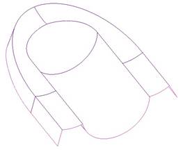
Now, we are going to create a mirror that goes around the top edge. Often, when you have a round that traverses a mirroring plane, it is better to mirror first, and then add the round. Therefore, we will click on the round tool, enter a radius of 0.25”, and then select on the following edge.
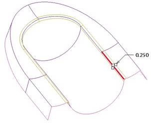
Once you create the round, select the entire quilt, followed by the Thicken tool. Enter a thickness of 0.125”, and point the direction to the inside of the surface, as shown in the following preview.
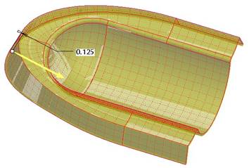
Finish the thicken tool, and our model will be complete, as shown in the next figure.
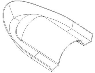
Save and close this model.
LESSON 33 – Layers
There are no exercises for this layer.
LESSON 34 – Parameters & Relations
Open up the Draft1 part. It should have a rib that is patterned five times (every 72 degrees). If not, start by patterning this rib. To do this, right click on the rib and select Pattern. For the pattern type, change it to Axis, and select the Z_AXIS. For the increment, enter 72 degrees, and a total count of 5.
The part with the pattern of ribs should look like the following.
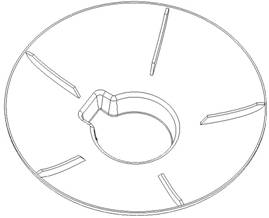
In order to drive the pattern, we will need to see not only the angular spacing between the ribs, but the number of ribs itself. Therefore, we will right click on the pattern in the model tree and select Edit. This will bring up the following dimensions.
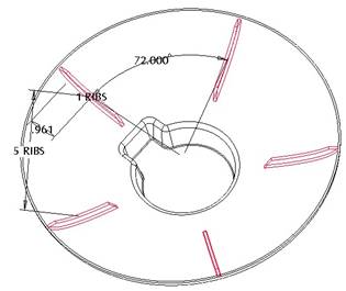
We can see the angular spacing (72.000) and the number of ribs (5). With these dimensions visible, go to Tools, Relations, which will cause the dimensions to temporarily switch to their symbolic names, as shown in the next figure.
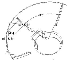
Therefore, to drive the equally spaced ribs based off of the number of ribs, the equation that we need to write (in words) would be:
Angular Spacing = 360 Degrees / Number of Ribs
Therefore, we must enter:
d33=360/p36
We have a window that opens for us to enter the equation, which currently looks like the following.
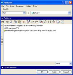
We will enter the equation exactly as we specified into this window, as shown in the next figure.
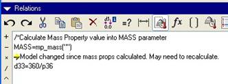
NOTE: Be sure to look at your model to see if your symbolic names are the same as this exercise solution, if not, you will need to enter the names as they appear on your model. Once you have entered the relationship into the window, click on OK. In the model, edit the pattern again, and change the number of ribs from 5 to 10, and then regenerate your model. You should see 10 equally spaced ribs, as shown in the next figure.
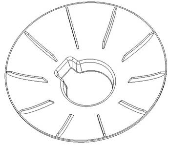
Save and close this model.
LESSON 35 – Family Tables
There are no exercises for this lesson.
LESSON 36 – View Manager
There are no exercises for this lesson.
LESSON 37 – Assembly Mode – Bottom-Up Design
Create a brand new assembly called Machine_Vise in the Machine_Vise folder. We have already created the sub-assembly called MV_Screw_Assy in this lesson, but we are going to create the top-level assembly now.
Component 1 – 01_MV_BASE
Click on the Assemble Component icon. When the Open window appears, select the 01_mv_base.prt component, followed by Open. This will bring the base model into our working window, and the Component Placement window appears. Since this is our first component in the assembly, we will click on the Defaut placement icon, followed by OK. Our first component looks like the following.
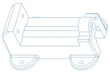
Component 2 – 02_MV_SLIDING_JAW
Click on the Assemble Component icon again. This time, select the 02_mv_sliding_jaw.prt component. When the placement window appears, we will start picking references according to the next figure.
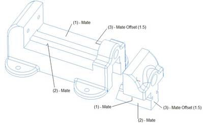
(1) – Mate
Select on the top flat surface of the 01_mv_base part, and the underneath flat side of the 02_mv_sliding_jaw component. Be sure the placement type is Mate with a Coincident type associated to it.
(2) – Mate
Select on the inner front surface of the 01_mv_base, and the front surface of the 02_mv_sliding_jaw component. Use another Mate, Coincident for the placement type.
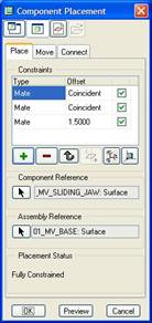
(3) – Mate Offset (1.5)
Select the inner left-facing surface on the 01_mv_base component, followed b component, followed by the right surface of the 02_mv_sliding_jaw component. An arrow will appear asking for the offset distance. Enter 1.5 if the arrow is pointing to the left. If the arrow is pointing towards the right, enter -1.5.
The component placement window should look like the following when all references have been selected.
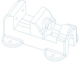
Click on OK, and the following figure shows the placement of this component.
Component 3 – 03_MV_SLIDE_KEY
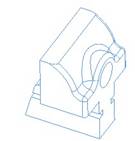
For this next component, it will be easier to hide the first component that we assembled. To do this, right click on the 01_MV_BASE component in the model tree, and select Hide. It will temporarily disappear from view, as shown in the next figure.
Click on the Assemble Component icon, and pick the 03_mv_slide_key.prt component. Use the references in the next figure to assemble this component.
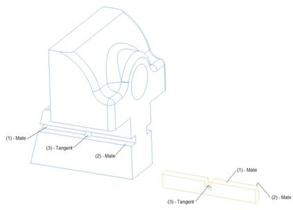
(1) – Mate
Select the back surface of the groove on the 02_mv_sliding_jaw component with one of the two side surfaces on the 03_mv_slide_key component. Make sure the constraint is a Mate with a type of Coincident.
(2) – Mate
Select the bottom of the groove on the 02_mv_sliding_jaw component, and the bottom flat surface (back in this figure) of the 03_mv_slide_key component. Use a Mate, Coincident constraint with this one as well.
(3) - Tangent
This one is sort of tricky. You may want to use Ctrl-Alt and the right mouse button to slide the key over until the square cut-out on the “03” component lines up with the hole on the “02” component, and then using a hidden line view, select one side of the cylindrical hole and one side of the square cut, thus producing a tangent constraint.
When done, the placement of this component looks like the following.
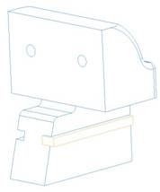
Component 4 – 03_MV_SLIDE_KEY
Repeat this same process to assemble the other slide key. The fully assembled key looks like the following.
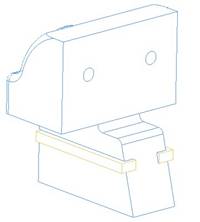
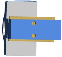
Component 5 – 04_MV_SET_SCREW
Assemble in the 04_mv_set_screw.prt component. Use the placement constraints shown in the next figure:
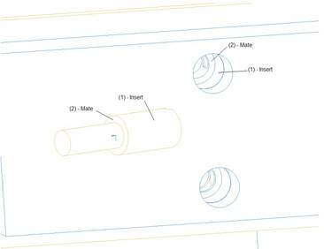
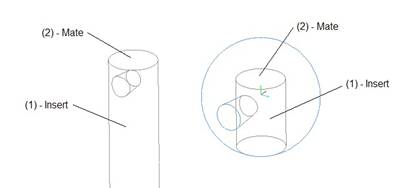
(1) – Insert
Select on the larger cylinder on the set screw and the inside surface of the hole on the bottom of the sliding jaw component. An Insert placement type should be created automatically.
(2) – Mate
Select on the middle flat surface of the set screw and the first noticeable flat surface you see in the hole on the bottom of the sliding jaw. Be sure to make the offset distance 0.0 and select a Mate command. It may come in originally as an Align Offset.
The final placement for the first set screw looks like the following.
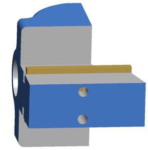
Component 6 – 04_MV_SET_SCREW
Repeat this process for the second set screw, whose placement looks like the following when complete.
Component 7 – 05_MV_JAW_PLATE
Assemble in the 05_mv_jaw_plate.prt component, and use the following placement references and constraints.
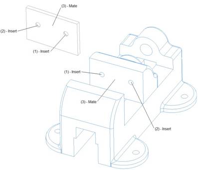
(1) – Insert
Pick on one of the holes in the sliding jaw and the corresponding hole on the jaw plate. An Insert command will be created.
(2) – Insert
Do the same for the other set of holes.
(3) - Mate
Pick on the flat part of the jaw plate that does not have the countersink around the holes and then pick on the flat surface on the sliding jaw. Be sure to use a Mate constraint with a 0.0 offset (or coincident).
Use Ctrl-Alt and the Right Mouse Button to move around the component as necessary for easier picking.
The final placement of this plate is shown in the next figure.
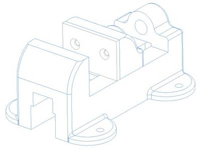
Component 8 – 05_MV_JAW_PLATE
Repeat this process to add another jaw plate to the stationary side of the base, as shown in the next figure.
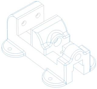
Component 9 – 06_MV_FLAT_HEAD_SCREW
Assemble in the 06_mv_flat_head_screw.prt into the assembly using the following two placement constraints and references.
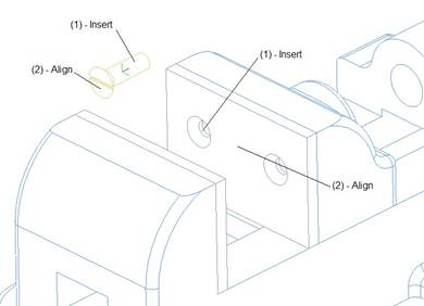
(1) – Insert
Select on the cylindrical surface of the screw and the first cylindrical surface of the jaw plate. An insert constraint will be created. Use Ctrl-Alt-RMB to move the screw so it is visible to select the next references.
(2) - Align
Pick on the flat head of the screw, and the flat surface of the jaw plate and use a coincident align to make them flush.
The final placement of the first screw is shown in the next figure.
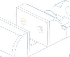
Components 10-12 – 06_MV_FLAT_HEAD_SCREW
Repeat this same process to bring in the remaining 3 flat head screws in the locations shown in the next two figures.
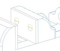
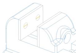
Component 13 – MV_SCREW_ASSY
The next component we will bring in will be the mv_screw_assy.asm assembly that we created in this lesson. We will use the following constraints for this assembly placement.
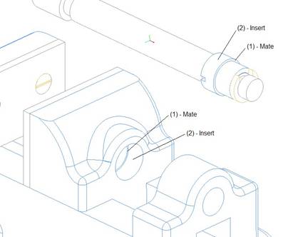
(1) – Mate
I chose to do the mate first so it would flip the assembly around to be facing the right direction. Pick the small flat surface in the middle of the collar and the first small flat surface you encounter in the hole on the sliding jaw. Change the constraint to a coincident mate.
(2) – Insert
Next, select the large cylindrical surface on the collar and the first cylindrical surface of the hole on the sliding jaw.
The final placement for this sub-assembly is shown in the next figure.
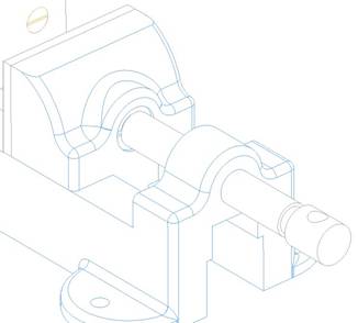
Component 14 – 10_MV_HANDLE_ROD
The next component will be the rod that goes through the end of the sub-assembly that we just placed. To do this, we will use an insert, and then a mate offset to fix the movement of this rod through the hole. The following figure shows these placements.
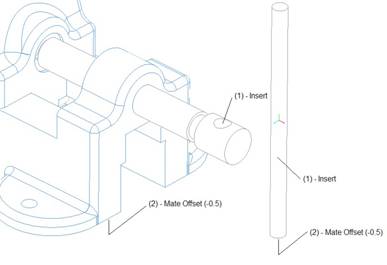
(1) – Insert
Select the cylindrical surface of the rod and the inside of the hole on the sub-assembly. An insert command should be created.
(2) – Mate Offset (-0.5)
Select on the bottom flat surface of the rod, and the bottom flat surface of the base. It may create a coincident align, so you will need to go into the placement window and use the pull-down to change it from Coincident to 0.0, and then edit this number to -0.5 to move the rod up.
The following figure shows this final placement for the rod.
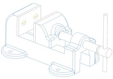
Component 15 – 11_MV_HANDLE_BALL
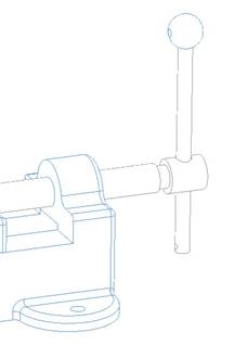
Assemble in the 11_mv_handle_ball.prt component. You may wish to turn on hidden lines to see the placement references easier. We will use the following references.
(1) – Insert
Select the cylindrical surface on the rod, and the cylindrical surface of the hole in the ball. An insert command will be created.
(2) – Mate
Select on the top flat surface of the rod, and the inside flat surface of the hole on the ball. Use a coincident mate for this placement.
The following figure shows this component’s placement.
Component 16 – 11_MV_HANDLE_BALL
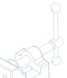
Repeat this process for the second ball. We will have to add a third constraint for this ball, because the holes for the taper pin will be on opposite sides when we use the same placement constraints as the first ball.
To rotate the ball around, uncheck the Allow Assumptions box in the placement window, and use Ctrl-Alt and the middle mouse button to rotate the ball around 180 degrees (approximately). Once the ball is rotated, click on the “+” symbol to add one more constraint. Turn on the visibility of datum axes, and select the two axes to Align to each other.
If you need to, re-select the Allow Assumptions box if the last constraint does not change the status to fully constrained.
The following figure shows this placement.
Component 17 – 12_MV_TAPER_PIN
Assemble in the 12_mv_taper_pin.prt component into the assembly. Turn on the display of hidden lines, and use the following constraints and references.
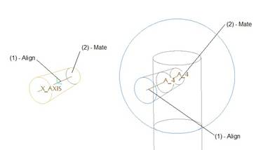
(1) – Align
Select on the axis of the taper pin, and on the axis of the ball. This will line up the axes using an Align constraint.
(2) – Mate
Select on the small flat end of the taper pin, and the inside flat surface of the rod and use a coincident mate.
Be sure the Allow Assumptions box is checked, and the following figure shows the final placement for this pin.
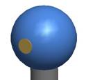
Component 18 – 12_MV_TAPER_PIN
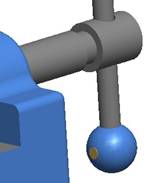
Repeat this process for the last taper pin, which will look like the following when assembled.
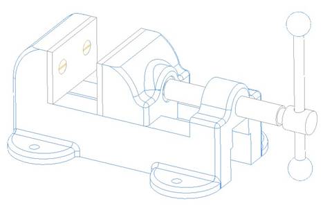
The following figure shows the completed Machine Vise assembly.
Save and close this assembly.
LESSON 38 – Assembly Mode – Top-Down Design
There are no exercises for this lesson.
LESSON 39 – Assembly Mode – Assembly Cuts
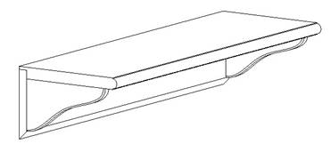
Switch working directories back to the ProETrain folder. Open up the assembly entitled Shelf.asm, which looks like the following.
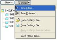
We need to create a series of assembly cuts to create the pre-drilled holes that will later be used for wood screws. Before we get started, go to your model tree, and select on the Settings button. When this expands, select on Tree Filters, as shown in the next figure.
When you select Tree Filters, you get the following window.
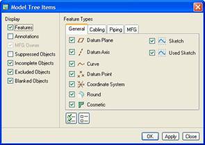
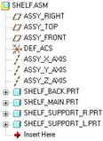
Select the Features option, as shown above, and then click on OK. Features will now be shown in the model tree, as we can see in the next figure.
Now, we are ready to begin. We will start with the holes on the back of the assembly. Click on the Extrude tool. When the dashboard opens, you should notice right away that the remove material icon is selected and grayed out, because we can only create cuts in assembly mode with this tool.
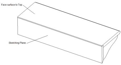
We will right click on the working window, and select Define Internal Sketch. When prompted, select the following references for the sketching plane, reference plane and orientation of the reference plane.
Inside the sketch, we will start on the right side of the part, and sketch 3 circles. Be sure all circles are assuming equal radii and lined up vertically. Dimension the circles as shown in the next figure.
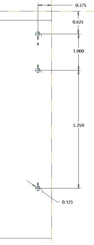
Now, zoom in on the left side, and sketch three more circles. For each of these circles, make sure they are using the same radii as the previous three, are lined up vertically with each other, and are lined up with their respective holes horizontally. We should only need one dimension for these three circles, as shown in the next figure.

Now, sketch two remaining circles in line with the top holes, using the same radii value as the others, and dimensioned from the left as shown in the next figure.

Once you have all eight circles sketched, click on the blue check mark to complete the sketch. Change the depth of the cut to 1.5, and the preview will look like the following.
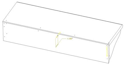
Before we go any further, expand the Intersect slide-up panel. It currently looks like the following.
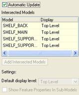
We do want the holes to intersect all of the parts in this assembly, so the list of models is correct, however, we want the visibility of the holes to be at the part level, and currently, only the top-level assembly is going to show them.
Therefore, we need to uncheck the Automatic Update box so we can control the values in the table. Once unchecked, pick on the Display cell that currently says Top Level, and change it to Part Level as shown in the next figure.
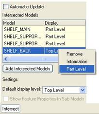
Do this for each of the model rows, until our slide-up panel looks like the following.
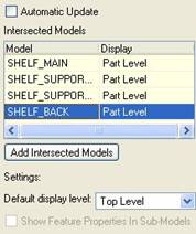
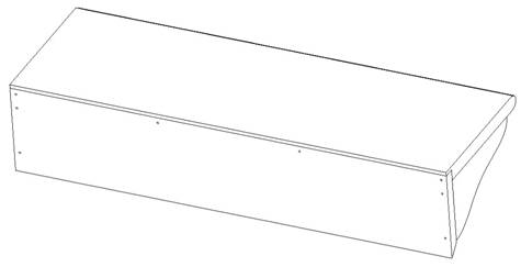
Now, we are ready to complete this extruded cut. Click on the green check mark, and our model will look like the following.
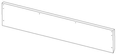
We can verify the display level by opening up the SHELF_BACK component, and we can see the holes in this part.
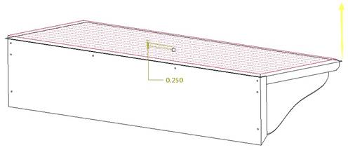
Before we create our new extrude, we will create a datum plane in the assembly. Therefore, click on the create datum plane tool, and select on the top flat surface of the assembly. Use -0.25 for the offset distance, to place it into the shelf, as shown in the following preview.
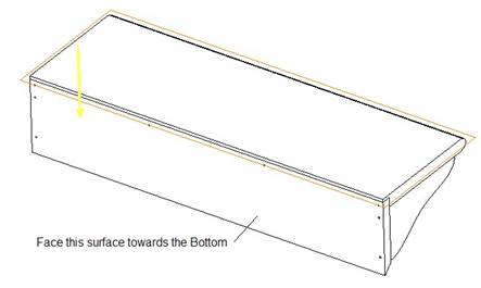
Click on OK, and we will now have an ADTM1 plane in our model tree. Now, we will click on the Extrude tool again. Use Define Internal Sketch to start our sketch, and select the ADTM1 from the model tree to use as our sketching plane. Make sure the direction of viewing is going down into the shelf, and then select the following surface to face towards the Bottom.
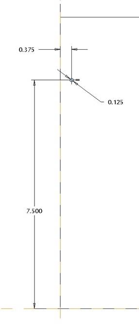
Inside the sketch, start on the left side, and sketch a circle dimensioned as shown in the next figure.
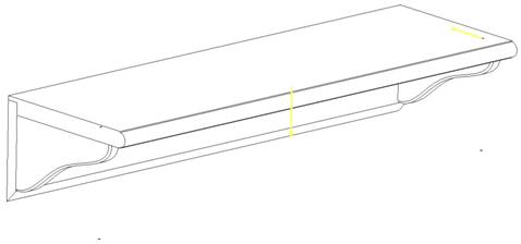
Then, sketch a circle on the right side that is the same radius as the first one, and lines up horizontally. Dimension it as shown in the next figure.

Click on the blue check mark to complete this sketch, and change the depth option to Through All, making sure the direction of feature creation is going down through the shelf. The following shows the preview at this point.
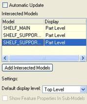
Open up the Intersect slide-up panel, which shows only the SHELF_MAIN and the two SHELF_SUPPORT models. This is correct, but we will need to uncheck the Automatic Update box to change each of these to Part Level visibility, as shown in the next figure.
Click on the green check mark to complete this second extrude feature. We can see the following in our assembly.
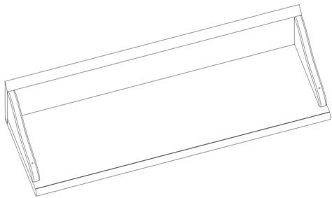
If we open up the SHELF_MAIN component, we can see the holes that were created by both extrude features.
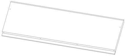
Save and close this assembly.
LESSON 40 – Assembly Mode – Assembly Operations
There are no exercises for this lesson
LESSON 41 – Drawing Mode – Drawing Fundamentals
There are no exercises for this lesson
LESSON 42 – Drawing Mode – Creating A Drawing
There are no exercises for this lesson
LESSON 43 – Drawing Mode – General Views
There are no exercises for this lesson
LESSON 44 – Drawing Mode – Projection & Section Views
There are no exercises for this lesson
LESSON 45 – Drawing Mode – Auxiliary & Detailed Views
There are no exercises for this lesson
LESSON 46 – Drawing Mode – Show Axes & GTOL Datums
There are no exercises for this lesson
LESSON 47 – Drawing Mode – Dimensioning
There are no exercises for this lesson
LESSON 48 – Drawing Mode – Broken & Partial Views
There are no exercises for this lesson
LESSON 49 – Drawing Mode – GTOLS & Symbols
Switch working directories over to the Drawing folder. Open up the drawing entitled GTOL_Create. It initially looks like the following figure.
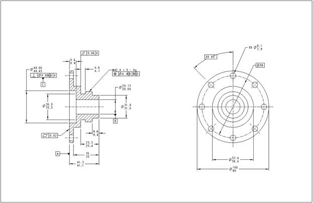
We will start by completing the two geometric tolerances on the cross-section view, which currently looks like the following.

GTOL 1 – Circular Runout
We will start with the Circular Runout tolerance on the larger of the two diameter dimensions on the right of this view. Therefore, go to Insert, Geometric Tolerance. When the window opens, click on the Circular Runout symbol (single arrow). This will make the screen look like the following.
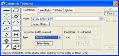
Keep the Reference type at Surface and then click on the Select Entity button. Pick on the cylindrical surface that highlights in blue when you place your mouse in the following location.
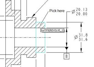
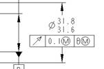
For the Placement type, keep Dimension, and click on the Place Gtol button. Pick on the 31.8/31.6 limit diameter dimension to the right of this view. We will see the GTOL appear on the dimension. Use Move to clean up the location. Currently, my control frame looks like the following.
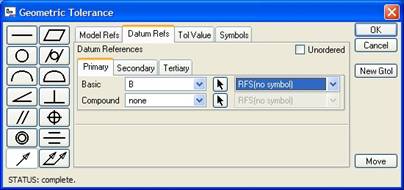
Now, we will click on the Datum Refs tab, and make sure B is the primary datum referenced. We should not have any material symbols set (RFS should be set), as shown in the next figure.
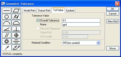
Click on the Tol Value tab, and change the tolerance to 0.1. Again, no material condition should be set, and our window should look like the following.
Click on the OK button to complete this tolerance. Our control frame looks like the following figure.

GTOL 2 – Circular Runout
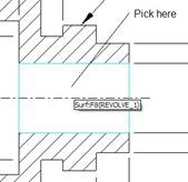
We will create another circular Runout. We could have clicked on the New Gtol button while we were in the last definition, but we did not, so we will have to go back through Insert, Geometric Tolerance. When the window appears, we should still have the same values as we did for the previous Runout. This time, click on the Select Entity, and pick in the location shown in the following figure.
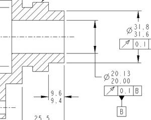
We will use the Dimension placement type, and click on the Place Gtol button to place the control frame on the 20.13/20.00 limit diameter dimension next to the one we selected in the last GTOL.
The control frame appears on the dimension, and the set datum “B” reference attaches to the bottom of it. We will use Move to clean up the location of the dimension, as shown in the next figure.
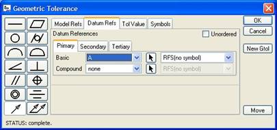
We will now edit the values. In the Datum Refs tab, make sure you are on the Primary tab, and select A for the reference, as shown in the next figure.
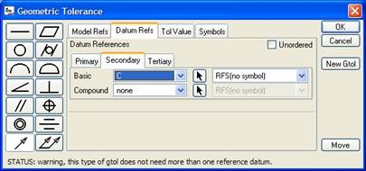
Now, click on the Secondary tab and select C as the datum reference, as shown in the following figure.
Now, click on the Tol Value tab, and enter 0.14 for the tolerance. We do not want any material conditions set, so our window should look like the following.
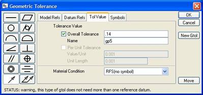
Click on OK to complete this GTOL, and our final section view looks like the following.
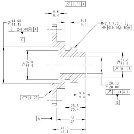
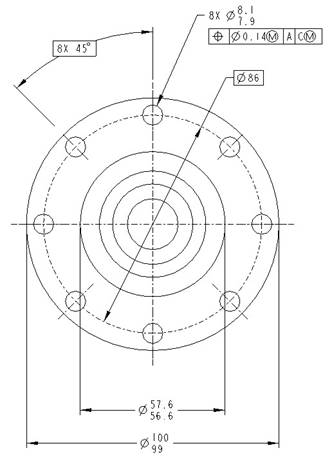
GTOL 3 – Position
The last GTOL that we need to create is on the RIGHT view. It will be a position tolerance. Therefore, click on Insert, Geometric Tolerance, and when the window appears, click on the Position symbol. Our window will look like the following.
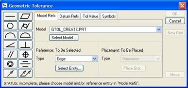
For the Reference type, change the option to Axis, click on the Select Entity button, and pick on the axis for the hole where the radius dimension is attached, as shown in the next figure.
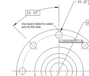
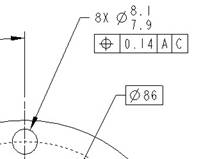
For the Placement type, keep Dimension selected, and using the Place Gtol button, pick on the radius dimension (8.1/7.9 limit dimension). We can see the control frame on the drawing view, as shown in the next figure.
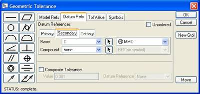
Go to the Datum Refs tab. The Primary tab should still show A, and the Secondary tab still shows C, but we need to add a maximum material condition symbol to the secondary reference, as shown in the next figure.
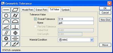
Now, go to the Tol Value tab, and add a maximum material condition to the tolerance, which should still be set at 0.14 from our previous GTOL definition, as shown in the next figure.
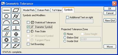
Go to the Symbols tab, and check the box for the Diameter symbol, as shown in the next figure.
Click on OK and our GTOL definition is complete. The completed view looks like the following figure.
Save and close this drawing.
LESSON 50 – Drawing Mode – 2D Drafting
There are no exercises for this lesson
LESSON 51 – Drawing Mode – Tables & Balloons
There are no exercises for this lesson
LESSON 52 – Drawing Mode – Adding Sheets & Finalize
There are no exercises for this lesson
LESSON 53 – Drawing Mode – 2D Drafting
There are no exercises for this lesson