|

Lesson Objective: In this lesson, we will learn about adding gravity to our mechanism models.
USAGE OF GRAVITY
Up to now, we have driven our assemblies using servo motors that define a distinct range of motion. Gravity has never come into play, but in order to model some mechanism connections, you will need gravity to create a realistic analysis and animation.
EXAMPLE 1 – BOUNCING BALL
Nothing demonstrates gravity as much as an object being dropped, and falling to earth of its own free will. We will now demonstrate how to set up a simple mechanism assembly to capture a ball bouncing.
Therefore, open up the assembly called Bouncing_Ball.asm, which looks like the following.
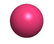
Yes, the assembly contains a single, ball part. We could have created a floor part, but that would have complicated things more than we needed. Instead, we defined the travel of this ball using a slider constraint.
Go to Applications, Mechanism, and you will see this slider, as shown in the next figure.
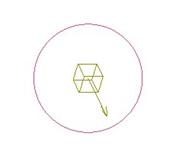
This slider is set up by taking an axis and plane from the ball and lining it up with an axis and plane on the assembly. So, you might be asking what prevents this ball from going through our “supposed” floor – or for that matter, where is the floor?
The answer is as simple as setting limits. If you look at the joint settings for this ball, you will see the following.
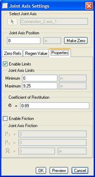
The ball is set to be dropped 9.25 inches off the floor, which is defined by the zero location (zero limit). Try dragging this ball around, and you will see that it truly does stop between two invisible planes. Why 9.25? The height we are starting at is actually 10” off the ground, but since the location of the ball is specified at its center, we needed to adjust our drop to ensure the diameter of the ball didn’t sink into the floor. The ball is 1.5” in diameter, hence the 9.25 drop to account for the .75 radius.
Make sure that the ball is set at the top of the limit (at the maximum height) – which in this case is “0”. NOTE: The positive direction of the slider is downwards, so 9.25 represents a drop of 9.25.
In the joint axis settings window, you will also see that a Coefficient of Restitution (e) has been set for this joint. If you recall from a much earlier lesson, an “e” value of 1.0 is completely elastic. A value of 0.0 is completely plastic – similar to dropping a ball of clay.
Therefore, we want to use something closer to the elastic range, but not perfectly elastic, or this ball will continue to bounce forever. Instead we chose 0.89.
Click on Ok to exit out of the joint settings. Notice that we did not have a servo motor defined? For a purely gravity induced analysis, no servo motor is needed, as long as we are using a Dynamic analysis, and we define gravity.
Gravity
On the feature toolbar, there is an icon that looks like the following.
![]()
We will click on this to reveal the following.
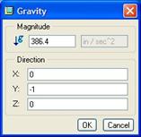
The value of gravity must be entered. It is approximately 386.4 in/sec2. The direction fields determine which direction the gravity is applied. In our model, gravity would go in the opposite as the positive “Y” direction, that is why it has a “-1” in this field.
Click on OK to finish out of this gravity definition.
Analysis
Now, we will go look at our analysis. Edit the Ball_Drop analysis, and you will see the following.
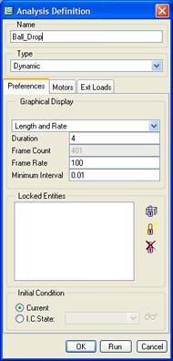
To capture a smooth motion of the ball bouncing, you will want to increase your frame rate. I also initially set the length of the analysis longer than I needed to determine how long the ball continued to bounce. It turned out that 4 seconds was enough time to see the ball lose its energy.
Click on the Ext Loads tab, and you will see the following figure.
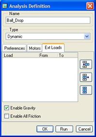
Here is where we enable gravity for this analysis. Note – we are using a Dynamic analysis in this case.
Click on Run to watch the ball move. Play your results back in slow motion to really see what is going on. To view a photo-rendered movie of this ball bouncing, open up the Bouncing_Ball.mpg file in your training directory.
Save and close this assembly.
EXAMPLE 2 – NEWTON’S CRADLE
Another perfect example of gravity is the Newton’s Cradle – a desktop toy that people have loved for years. Therefore, open up the assembly entitled Newton_Cradle.asm. It will look like the following.
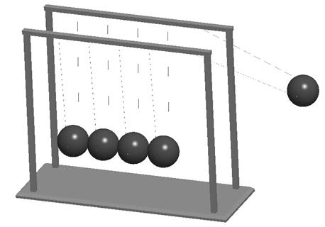
This assembly consists of a base part (the frame of the cradle), and a ball (with simulated string), assembled five times.
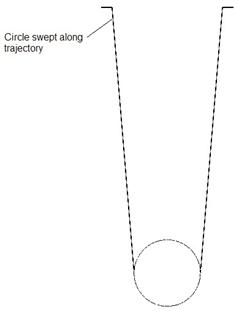
The string is actually a swept protrusion that looks like the following.
Setting Up The Assembly
Each ball part is assembled using a pin connection that takes one of the free ends of the swept protrusion and inserts it into a hole on the base frame. Each ball is free to rotate. There are no server motors set up, but we did create four cam followers, one to allow for impact between each of the five balls.
Each ball has a circular sketch feature that was selected for the cam curve. If we go to Applications, Mechanism and look at a front view, we can see the pin connections and the four cams.
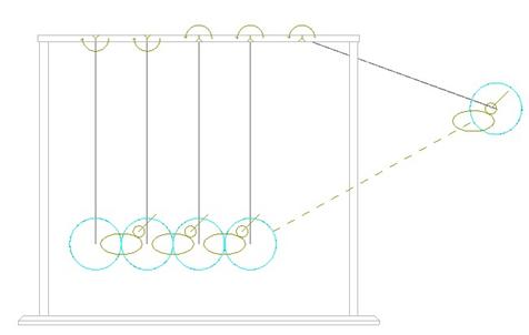
The right-most ball is set out at an initial starting angle on the pin constraint as if we had pulled it out.
Cam Followers
Each cam follower has the following Properties tab defined.
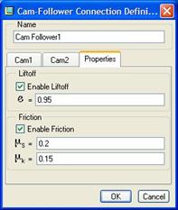
We enable liftoff so the balls can separate and bounce off each other, and we set a coefficient of restitution to 0.95 to try to get as close to an elastic collision as possible (force is nearly completely transferred from the moving ball to the ball it impacts).
We also set some friction coefficients to allow some of the energy to dissipate as the balls rub against each other.
Analysis Definition
If we look at the analysis (NC_Motion), we see the following.
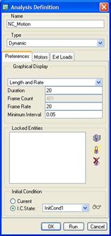
A snapshot was created that is used for the starting position. The trick in getting the energy to pass to each of the balls is to provide for a very slight separation of the balls, which is captured in this snapshot. In the real Newton’s Cradle, the balls hang in such a way that they touch each other. In Mechanism, if we did this, all of them would act like a single mass.
If we click on the Ext Loads tab, we see the following.

We can see that we have enabled gravity and all friction definitions. If we don’t enable friction, then it will ignore the friction coefficients that were set up in the cam followers.
Last Considerations
We need to make sure that we define the density for our balls, as the impact force of the falling ball will vary greatly if we use the default density of 1.00. We used the density of 304 Stainless Steel.
Run the analysis, and you will see the simulation of Newton’s Cradle. This demonstrates a great use of cams, friction and gravity combined to give a realistic animation. If you would like to see a photorendered movie for this analysis, open up the Newton_Cradle.mpg movie file in your training directory.
Close this assembly when you are done.
LESSON SUMMARY
Gravity can be used to enable dynamic analyses when no servo motor or external force can be defined.
EXERCISE
Open up the assembly called Ferris_Wheel.asm. All of the mechanism connections have been set. All you need to do is create an analysis that will run for 60 seconds that simulates the ferris wheel going around. Use the existing servo motor. To see a completed movie, open the Ferris_Wheel.mpg file in the training directory.