Lesson

4

Lesson Objective: In this lesson, we will take a small step into understanding ISDX curves, and how to manipulate them.  We will also learn about Curve Curvature.

ISDX CURVE INTRODUCTION

Even if you don’t need to create an ISDX surface, you may find yourself wanting to use ISDX curves in place of other datum curve types for the ease of creation and flexibility of change properties that they possess.

Simply stated, there is no other curve tool in Pro/ENGINEER that can occupy 3D space without needing either a custom sketching plane or a series of individual curves that can be combined or intersected to form the final curve.

You have the ability to make rapid changes to ISDX Curves, and control tangency and curvature conditions very easily with ISDX curves.

SIMPLE EXAMPLE

To demonstrate the ease of creating a 3D ISDX curve, we will look at a simple example of a curve that passes between two vertices on a part.  We will start by opening up the part file entitled 2Point_Curve.prt.  It will initially look like the following.

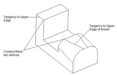
We are going to create a curve that connects the two vertices shown in the following figure, and we want the curve to be tangent at each end to an adjacent edge, also shown in the figure below.

Traditional, Non-ISDX Method

We will first create this curve using traditional Datum Curves.  Therefore, click on the following icon.

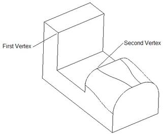
When the menu manager appears, we will select the Thru Points option, followed by Done.  When the feature window appears, we start by clicking on the points that the curve goes through.  Pick the two vertices in the order shown below.

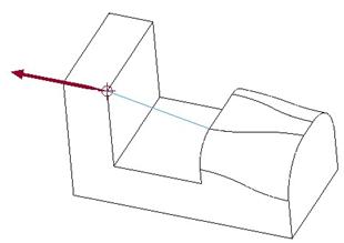
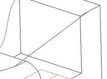
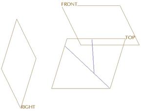
Once we pick the second vertex, we will see a line appear with a blue arrow, as shown below.

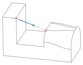
Once we see this, click on Done from the menus.  We should see an outline of a straight line between the two vertices.  To see it more clearly, refresh your screen, and then click on the Preview button.  This will make the blue line appear with the blue arrow indicating the start location for the curve.

Now, we are going to double-click on the Tangency element in the feature window to define this.  We are initially placed into defining an edge to determine tangency for the start point, as we can see from the menu at the top of the next page.

We want to pick the straight edge shown below.

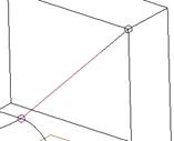
Once we select this edge, we will see a maroon arrow appear as shown below.

This arrow indicates the direction the tangency is determined from.  We want to flip it if it looks like the figure above so the arrow is pointing towards the open space.  Once you flip it, click on Okay, and we will see the curve update.  We are then placed into defining the tangency edge for the end point, as shown at the top of the next page.

Select the edge indicated above.  Another maroon arrow will appear on the model, and we want it to go in the direction shown in the following figure.

Once the arrow is going in this direction, click on Okay, followed by Done/Return to finish out of this tangency definition.  Click on OK from the feature creation window, and our curve will look like the following.

This is a perfectly acceptable way of creating a 3D curve that passes between two vertices.  By specifying the tangency condition, we ensure that any surface that we create will have a smooth edge transition.

ISDX Method

This time we will create the same curve using ISDX.  We will start by clicking on the ISDX tool in the feature toolbar, as shown below.

Once we see the ISDX toolbar, we will click on the Create Curve icon, which looks like the following.

When the dashboard appears, we will make sure the type is specified as Free, as shown below.

Free is the option used to create a curve that does not lie in a 2D plane, and is not projected onto a surface of the model.  We will begin by holding down the Shift key on the keyboard, and then place our mouse over one of the edges that we want to tie to, as shown below.

We know we are over the edge when we can see a “+” symbol appear at the end of our mouse cursor.  Holding down the shift key enables us to snap to existing geometry.  Once we see the “+” symbol, click with the left mouse button, and we should see an open circle appear on that edge where we selected, as shown at the top of the next page.

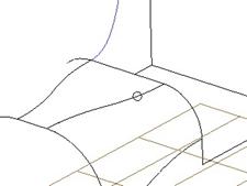
Now, hold down the shift key again, and select on the other edge to tie to, as shown in the following figure.

Once you see the “+” symbol on this edge, click with the left mouse button, and you will see the curve that we are creating, and another open circle at the location where we picked.

If you remember from Lesson 2, when you see an open circle at the end of a curve, it is called a Soft Point.  This means that the end of our curve lies on the edge selected, but it can translate along the edge.

You might be wondering why we didn’t just pick on the vertex like we did with the traditional approach.  The reason for that is because we need to determine which edge will drive the tangency condition that we are going to set.  Each vertex has three entities that meet at the vertex.  There is a way (if you practice it enough) to not only snap directly to the vertex, but to also determine at the same time which edge you are using.  Until you are comfortable with ISDX, I would recommend doing it the way we did here.

Now that we have the two endpoints defined, click with the middle mouse button to complete this curve.  The circles should disappear, and we should just see our curve, as shown below.

The curve tool remains active, allowing us to create as many ISDX curves as we need.  We are going to switch over to the Edit Curve command by clicking on the following icon.

If your curve does not automatically highlight in red with both of the circles present, then click on it to activate it.  Now, we will drag the first end of the curve until the open circle stops at the vertex, as shown below.  Do NOT hold down the shift key, or you will make the circle come off the edge.

Now, do the same for the other endpoint until it sits at the vertex shown at the top of the next page.

While we have this second end selected, we can see the yellow tangency line that appears on the vertex, as shown below.

We will hold the right mouse button down over this tangency line to see the list of options.  We will select the Tangent option, as shown below.

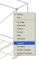
This forces the curve to be tangent to the line that it is currently sitting on (the one that we attached it to in the first place).  The curve will update to reflect the tangency, and an arrow will appear on the model indicating the direction of influence for the tangency condition, as shown below.

If it was possible to flip the direction of influence, you could just click on the arrow and it would flip.  Unlike traditional datum curve creation methods, it understands when you can not flip it (or when it does not make sense to do so).  Since there is only a single ISDX curve touching existing geometry, the tangency condition can only be applied in one direction, from the existing edge into the curve, as indicated in the previous figure.

Now, we will repeat this same process for the other end.  We will start by picking on the other open circle to activate it and see the tangency line.  Right click on this tangency line and select Tangent again from the list that appears.

Once the arrow appears, click on the middle mouse button to accept this change to the curve.  We will now see our final curve.

Another major difference between the ISDX tool and the traditional approach to creating this curve is that we are still able to create additional curves at this time, and surfaces – all in a single feature.

We, however, are done at this time.  Therefore, click on the following icon to complete the ISDX Style feature.

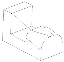
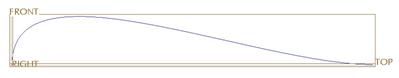
Our curve will appear in blue on the model, and a style feature will appear in the model tree.  Go to a FRONT saved view, and you will see that both curve methods produced identical results.

CURVATURE for CURVES

When you create a style curve, you can display its curvature plot.  To demonstrate this, open up the part file entitled Curvature.prt.  It should open up in the FRONT view, as shown below.

Turn off the datum plane display, and edit the definition of the style feature in the model tree.  Once you enter into Style mode, click on the following icon in the system toolbar to view curvature plots.

This will bring up the following window.

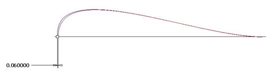
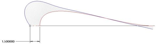
Select on the curve.  A curvature plot will appear on the curve, as shown below, along with a dimension.

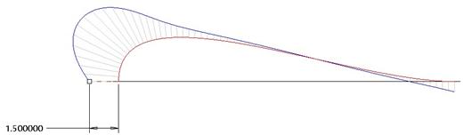
To adjust the size of this plot to see it easier, change the dimension value to 1.5, which will make the curvature plot look like the following figure.

Our Curvature window shows us the Max and Min curvature for our plot, as shown in the next figure.

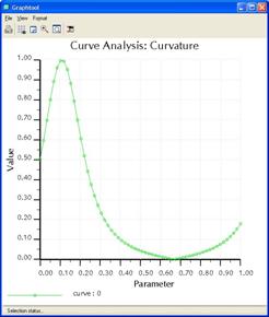
We can view a graph of the curvature over the length of curve if we click on the top icon on the right side of this window.  The result is shown in the following figure.

To change the density of the lines on the plot, we will click on the Definition tab in our window.  It looks like the following.

We will change the Quality field from 2.00 to 5.00.  This makes our plot look like the following.

Reading the Plot

So, how do we read this plot?  We know that our curve is internally tangent along its entire length, but it goes through transitions of curvature.  When the plot is far away from the curve, it indicates an area of high curvature.  When the plot is close to the curve, it indicates an area of low curvature.  If the plot lies on the curve itself, there is zero curvature for that area.

Understanding this, we can read the plot as follows.

Having areas of high, low and zero curvature does not mean we have a bad curve, it just means that we have something other than a straight line.  What we want to avoid is abrupt changes in the curve, which results in a dip or bump in the curvature plot.  Click on the green check mark to complete this curvature plot.

To demonstrate an abrupt change in this curve, we will first add a midpoint to this plot.

Adding a Midpoint

We will start by clicking on the curve edit tool (  ), and then select on the curve to highlight the endpoints.

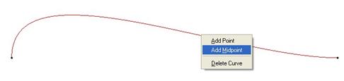
Next, we will right mouse click over the curve and select the Add Midpoint option, as shown in the following figure.

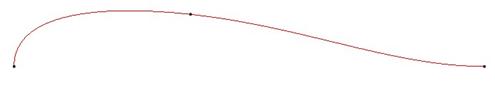
Another point will appear on the curve at its midpoint, as shown below.

Using the left mouse button, drag this midpoint up so it looks like the figure below.

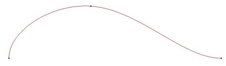
As you can see from the previous figure, there is a very abrupt change in curvature at the top of this curve where the midpoint is, as indicated below by the bump when we view the curvature plot again.

Ideally, a curvature plot should be smooth.  Any dips and bumps in the plot are signs that the curve has this rapid change in shape.  A dip or bump in the plot does not mean that there is a bump or dip in the curve itself, as it maintains full internal tangency.

CURVE POINT CONTROL

One of the advantages of working with Style curves is the ability to work unconstrained and un-dimensioned.  You can focus primarily on the shape of the model.  There are times, however, when you may want to control the actual location of an endpoint of a curve or internal point on a curve.

Style curves give you the flexibility of both.  To demonstrate this, we will open up the model entitled Point_Control.prt.  It will initially look like the following.

There is a single style feature that has been created that consists of two curves.  Edit the definition of this style feature.  Once inside the feature, we will begin by clicking on the curve edit tool (  ), and select the longer of the two curves.  Both ends should highlight in a small filled dot, as we can see in the next figure.

The small filled dot represents either an internal point (such as a midpoint), or an endpoint that is free (not connected or tied to anything).

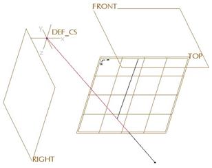
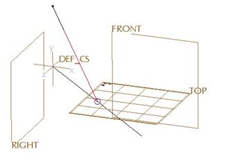
Using the orientation shown above (Default view), click on the leftmost endpoint to activate it.  You should see the tangency line appear at this end.  In the dashboard, click on the Point slide-up panel, which looks like the following.

In the middle of this window, we see a section entitled Coordinates.  The X, Y and Z values are based off the global coordinate system (DEF_CS) at the intersection of the three default planes (FRONT, TOP and RIGHT).  Therefore, if we wanted our selected endpoint to lie at the intersection of these three planes, we would change the X value from 5.0 to 0.0 and the Z value from 3.0 to 0.0.  Make these changes, and you will see the result, shown in the following figure.

On this same curve, select the other endpoint.  While the Point slide-up panel is still open, we can see the location of this point as X=12.0, Y=0.0 and Z=9.0.  Change the Z value to 12.0, which results in the next figure.

Now, click on the other curve to activate it.  We should see a soft point (large, open circle) where this curve meets the first one, indicating that the endpoint is free to move along the curve, but it is tied to it.

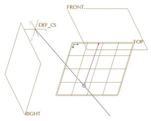
Click on the soft point, and the Point slide-up panel will look like the following.

We can see that we can not control the actual coordinates of this end point, because it is tied to the other curve.  We can, however adjust its location based off of values at the top of this panel.

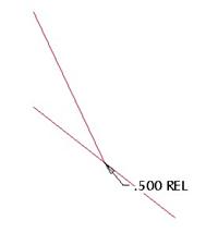
Right now, we are sitting at a Length Ratio of 0.65, or 65% along the length of the curve (measured from the left end).  If we wanted to place the soft point at the exact center of the first curve, we would change the value to 0.5, and we would get the following result.

Within this Soft Point section, we can use the pull-down field to see other options.  These are:

· Length Ratio – This is the default.  Measures the point along the curve at a percentage of its length.  The location is based on the “Physical” curve definition.

· Length – Defines the exact length along the curve from one of the endpoints.

· Parameter – This is similar to the Length Ratio, but is based on the “Mathematical” curve definition.  I recommend using “Length Ratio” over this option.

· Offset from Plane – Determines the position of the point on the curve at a distance from a selected datum plane or planar surface.

· Lock to Point – Locks the soft point to the closest internal point or endpoint, making it become a fixed point (shown with an ”X” symbol instead of an open circle).

· Linked – This indicates a state, not an action.  Our point is already linked with the curve at the soft point.  No other soft point types listed here are available if this option is selected, and therefore is not applicable in this example.  Other possible linked conditions are a soft point that lies on a surface or plane, or a soft point tied to a vertex or datum point.

· Unlink – Removes the link between the endpoint and the curve, causing it to become disconnected.  The open circle is then replaced with a closed dot, just like our free ends.

We will leave this soft point at 50% of the length of the curve.  You can also see a little check box next to the Value field.  If you check this box, you are making the value available to edit outside of the style feature.

Therefore, click on this box so a check appears, as shown below.  We will come back to this at the end to see what it gives you.

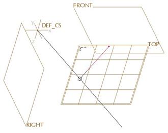
Finally, pick on the free end of the smaller curve, and change its coordinates to the following:

X=0.0

Y=5.0

Z=0.0

The result is shown below.

You can see from this short exercise that we have the ability to define exact locations for curve points (both endpoints and internal points – which we don’t have in this example).

Go ahead and click on the blue check mark to finish out of the style feature.  Now, we will right mouse click on the style feature in the model tree and select Edit.  We should see the Length Ratio value that we specified using the check box.

We can now modify this value just as we do any other dimension in Pro/E and regenerate the model to see the change.

LESSON SUMMARY

When creating 3D curves in Style, you can control the location of the endpoints by entering exact x, y, or z coordinates, or snapping to existing geometry, such as an edge, surface or vertex.

EXERCISE

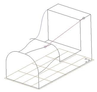
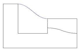
Open up the model Transition.prt, which should look like the following.

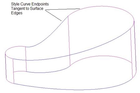
We want to create a single style feature that contains four separate curves.  Each curve will connect one vertex of the smaller surface with its corresponding vertex on the larger surface.  Be sure to set tangency conditions with the endpoints of the curves with their corresponding surface edge to get a nice smooth transition, as shown in the final result below.

Save this part for the next lesson’s exercise.